
Frequency oversampling
"All models are wrong, but some are useful"
George Box - 1976
When modelling, we're always simplifying nature in order to answer some generalised questions. However, sometimes we also simplify in order to save resources, more specifically save (CPU) time. dBSea (and many other propagation models) do no calculate propagation loss for the whole frequency range, but rather calculate the propagation loss for a small subset, usually every third octave.
 |
| Table 1. Nominal octave and third octave bands. |
For simple scenarios this approach is not going affect results too much (compared to other contributors of uncertainty), but for rough seabeds, it makes quite a lot of difference. When sound interacts and reflects off a sediment the wavelength influences how this reflection, and resulting scattering plays out. Thus the frequency is important for the accurate calculation of propagation loss from bottom interactions.
I ran a few shallow water scenarios with a downward reflecting sound speed profile to illustrate this effect:
There is a clear change in predicted levels when changing oversampling from no oversampling (1x) to 10 times oversampling (10x), of ~6 dB on average. When increasing the oversampling further, gere to 20 times (20x) we only see a small change in the predicted levels (~1.5 dB). The change in predicted level VS oversampling rate thus seems to follow a general inverse power relation:
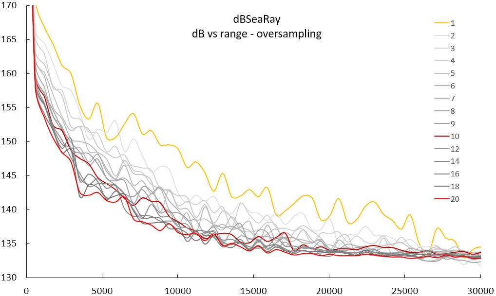 |
| Figure 1. Levels VS Range for frequency oversampling of 1x to 20x. Note the large change from 1x to 10x (~6 dB), but small change from 10x to 20x oversampling (~1.5 dB). |
y = ax^b Eq 1.
We set "y" as the level we see at a small oversampling rate, minus the level we would see at the limit where we no longer see a change in levels when we increase the oversampling rate.
"y" is now the difference between observed level and level at limit.
"y" is now the difference between observed level and level at limit.
For this particular case i got the following relation:
difference = 10*(x^-1) = 10/x Eq 2.
The "x" being oversampling rate.
And in graphic form:
And in graphic form:
 |
| Figure 2. The diminishing accuracy return of additional oversampling. Vertical axis is difference from ideal solution, while horizontal axis shows oversampling rate. |
Say we are happy with a 1 dB difference/uncertainty, we can solve Eq 2. for a difference equal to 1 dB and get:
1 = 10/x
x = 10
We should thus set our oversampling to 10 times for this scenario, to approximately have 1 dB of uncertainty from the oversampling rate.
Note for stat geeks: These and other uncertainties can compound, and should be kept in mind when evaluating your modelling results. If you assume the uncertainties are random, then the central limit theorem applies (making these deviations normally distributed), and you can truly unleash your inner statistician! (any folks out there with a liking for R-stats?).
Thanks for reading, and please comment if you like.
cedeiinru Brad Hill https://wakelet.com/wake/Zmh6q3TfQCMeP2S2GSn-O
ReplyDeletegaipsychappe
insalPlio-ra Sandy Zauner Reg Organizer
ReplyDeleteVMware Workstation
DesignCAD 3D Max
taacatgelern