Feature sneak peak
We've been working hard to move dBSea along, and while we're still working on making the 3D solvers ready, we've almost finished another feature that we quite like, and hope that you will too.
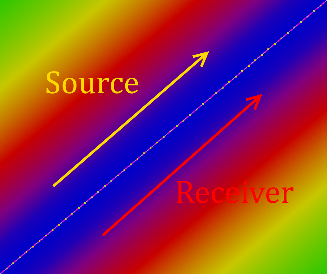
We now have a working alpha version of moving receivers, allowing for a much better estimation of animal impact by probing realistic routes used for daily foraging or seasonal migration.
 |
| Figure 1. Example of moving receiver (purple) and stationary source (light blue). |
We've also added a few tools to make data extraction easier, the first of which is a simple received level over time. If you set dBSea to remember all source positions then the individual movement of source(s) and moving receivers will be taken into account. In figure 2 the source is stationary, while in figures 5,7 & 9 the source is moving.
 |
| Figure 2. The received sound level over time for the receiver in Figure 1. |
In the defaults settings dBSea shows you the maximum level at any depth at each position. The moving receiver lets you view the variation in level with depth at each point. In figure 3 the depth-vs-level is shown, with green lines being the first points, and red the last.
 |
| Figure 3. The level versus depth at all receiver positions. Bright green is start of track, red is end of track. |
Setting up the path i similar to setting up the path for a moving source, with options to add points manually, or import CSVs or GPX files of the desired movement.
 |
| Figure 4. The motion of the moving receiver is set by entering easting and northing of waypoints, by importing GPX files or by dragging waypoints to their desired position. |
Moving receiver and moving source in a large scenario:
 |
| Figure 5. Source (yellow and blue) traveling through strait of Gibraltar and up Portuguese coast. Receiver (green) travelling south with sinusoidal dive profile at 2 m/s. |
 |
| Figure 6. Level versus time for the path in figure 5. Notice the pattern in levels corresponding to a diving frequency of 1 dive/hour, as well as lower levels when seamounts are between source and receiver. |
The following illustrations might better explain the effect of accounting for the relative position and time of both source and receiver.
First for source and receiver travelling the same way at the same speed.
We are almost done with testing of this new feature, which proved to be a lot more tricky to make than anticipated.
Thanks for reading, and please don't hesitate to leave a comment or a question.


Comments
Post a Comment